Home > News > Nobleo article on Actuator Matrix Design for Over-Actuated Systems

Nobleo article on Actuator Matrix Design for Over-Actuated Systems

Published on 30 Apr 2024

30 Apr 2024

High-tech positioning systems require high controller bandwidths and the decoupling of the various degrees of freedom (DoFs) to obtain the best system performance. Typically, one actuator is needed per actively controlled DoF, but practical design considerations often lead to an over-actuated system. It is shown here, however, that the freedom provided by over-actuation can be used to not only decouple rigid-body modes, but also to isolate non-rigid-body resonance modes. Thus the performance and/or robustness of the controlled system is improved without actually having to add an additional control loop.

Introduction

High-tech positioning systems aim to position a system very accurately. This often goes hand in hand with high velocities and accelerations. High controller bandwidths and mutual decoupling of the various degrees of freedom (DoFs) are desirable for obtaining the best system performance.

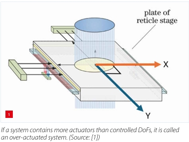
Typically, one actuator is needed per actively controlled DoF. Volume conflicts, design choices (such as symmetry for centre of-gravity positioning) or actuator force limitations often lead to an over-actuated system. In these systems there are more actuators than actively controlled DoFs (and sometimes even more actuators than observable DoFs); see Figure 1.

In motion control, the goal is usually to control the rigid body movements, i.e. the actively controlled DoFs. This is done by decoupling the MIMO (multiple input, multiple output) system into logical directions through combining physical actuator forces in such a way that a resultant force is applied in only one specific logical direction.

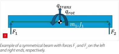
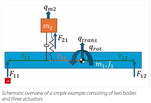
As an example, consider a symmetrical beam with two
DoFs, a translation and a rotation, and actuators on the left and right ends of the beam; see Figure 2. Typically, the sum of the actuators drives a translation and their difference the rotation, i.e., for translation, the two forces have the same direction and, for rotation, the opposite direction. This mapping can be captured in a distribution matrix, which is referred to as actuator matrix. This decoupling matrix is often based on geometry, mass and inertia properties of the system and decouples to the principal axes of inertia.

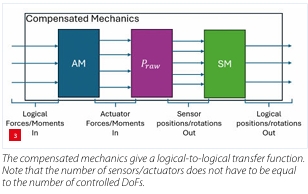
In a similar way, the sensor matrix converts sensor readings to logical coordinates. The mathematically obtained dec oupled system is referred to as compensated mechanics (see Figure 3). The term ‘compensated’ is used to distinguish between ‘raw’, i.e. physical, inputs/outputs and a system with AM and SM that works in logical (control-oriented) inputs/outputs:

𝑷_𝐂M= 𝑺M ∙ 𝑷_𝐫aw∙ 𝑨M

Here, P_CM is the compensated mechanics plant, SM is the sensor matrix, P_raw is the ‘raw’ plant, and AM is the actuator matrix. Thus, using an actuator matrix and a sensor matrix together with the ‘raw’ plant, the compensated mechanics are obtained. This transfer function describes the system in logical/functional DoFs. If the DoFs are along inertial axes this can also result in decoupled system behaviour, which then turns the control problem into a series of (decoupled) SISO (single input, single output) control tuning problems. Typically, this is the preferred route for the control design of high-performance mechatronic motion systems.

The actuator matrix maps the input signals to the physical actuators in such a way that only one functional input direction is actuated. All other specified directions should not be affected. Consider the beam shown in Figure 2; when this system is decoupled correctly, rotations can be made without making a translation and vice versa.

A practical method to derive the actuator matrix AM (for rigid-body-mode decoupling) is to use a measured transfer function from physical actuator inputs to logical outputs TF_raw(ω) = SM ∙ P_raw(ω) and define a frequency point at which the transfer function is mass-dominated (typically a low-frequency point), ^ω_mass, in a high-coherence (> 0.9) area, then:

$M_{\text{inv-meas}} = TF_{\text{raw}}(\omega_{\text{mass}})\cdot \omega_{\text{mass}}^{2}$

Assume now an ideal transfer function (inverted mass matrix) in the functional direction, i.e. along inertial axes, M^–1 (this matrix need not be exact, but it is always square and usually diagonal). To obtain the actuator matrix, the following equation can then be used:

$M_{\text{inv-meas}} \cdot AM = M^{-1}$

From which follows:

$AM = M_{\text{inv-meas}}^{-1} \cdot M^{-1}$

If a system contains as many actuators as controlled DoFs, the measured mass matrix ^M_inv–meas will, if all motions can be achieved, be a square, full-rank matrix. As a result, the actuator matrix AM will also be square and unique.

With an over-actuated system, there are more logical inputs (transfer function columns) than system outputs (rows). In such cases, the measured matrix ^TF_raw(^ω_mass) is not square and there is not one unique AM that can solve Equation 1. Here, the matrix inversion is often done using what is known as a pseudo-inverse. The pseudo-inverse calculates an optimal (minimum-energy) result, which is a solution AM = ^M_inv–meas^–1 ∙ ^M_inv, but not the only one! The solution space of all possible solutions to this equation can be calculated. In linear algebra, this is related to the null-space of ^M_inv–meas^–1, which is then not empty.

Physically, this means that there are multiple actuator distribution combinations possible for obtaining the desired effect of diagonalisation, i.e. decoupling. In the case of the beam mentioned earlier (Figure 2), if there were a third actuator, then the system would be over-actuated. There would be multiple combinations possible for the distribution of the forces over the actuators such that only a rotation or a translation is obtained.

This article provides an opportunity to use this design space to not only decouple rigid-body modes, but also to isolate non-rigid-body resonance modes. It is shown here that the freedom provided by over-actuation can be used to improve the performance and/or robustness of the controlled system, without actually having to add an additional control loop. As an example, by isolating non-rigid body modes, a bandwidth-limiting resonance can become ‘invisible’ for the rigid-body input. It could also be that tracking performance and settling improve, as the disturbing nonrigid-body modes are either not or less excited.

To do this analysis, a simple and practical example is used, which will be presented first. Then the theory of this method is discussed and how it can be applied to the simple example. Following the theoretical approach, the practical approach will be applied to the example. After presenting the simple example, the results for an existing, more complex system will be discussed. Finally, this article will draw some conclusions.

Simple Example

The simple example used in this article is that of a two mass-spring-damper system as shown in Figure 4. The goal is to control the two rigid-body states [q_trans q_rot]. The system has three actuators, two of which are positioned on the lower body with mass m₁ and inertia J₁, and one of which is on the upper body with mass m₂. For simplicity, it is assumed that the spring with stiffness k is only a translational spring and that the upper body has no rotational inertia. In this example, we can see directly that this is an over-actuated system and that there are different distributions possible that will achieve the goal of controlling the two rigid-body modes.

We will now show that the design space spanned by the over-dimensioning can be used to get a beneficial decoupling.

Theoretical approach

In the theoretical approach, we assume that the spring stiffness and all masses and positions with respect to the centre of gravity are known. The system can be described with three DoFs (two translations and one rotation). From this, the mass matrix ^M_model and stiffness matrix ^K_model can be derived:

$M_{\text{model}} = \begin{bmatrix} m_1 & 0 & 0 \\ 0 & J_1 & 0 \\ 0 & 0 & m_2 \end{bmatrix}$

$K_{\text{model}} = k \begin{bmatrix} 1 & r_{21} & -1 \\ r_{21} & r_{21} & r_{21} \\ -1 & -r_{21} & 1 \end{bmatrix}$

Here, the coordinate vector is:

$\vec{q} = \begin{bmatrix} q_{\text{trans}} \\ q_{\text{rot}} \\ q_{m2} \end{bmatrix}$

In order to isolate the three distinct eigenmodes, we transform the system into a modal representation with modal coordinates. From the K– and M-matrices it is possible to obtain the eigenfrequencies Λ and eigenvectors V (Matlab: eig(K,M)). Furthermore, it is possible to calculate the input transformation matrix H. This matrix describes how each actuator force input acts on each eigenmode.

Writing the compensated mechanics in terms of eigenvectors and the input transformation matrix gives:

$P_{\text{CM}} = SM \cdot V_{o} \cdot \Lambda \cdot V_{l}^{T} \cdot H \cdot AM$

Here, ^V_o is the eigenvector matrix for the output nodes (sensors), Λ is the diagonal eigenfrequency matrix, and ^V_I^T is the transposed eigenvector matrix for the input nodes (actuators). These follow from an eigenvalue, eigenvector or modal decomposition of the system. For the example discussed in this article, the two matrices are identical. The entries of matrices ^V_o and ^V_I can be interpreted as the modal contributions for each mode at the physical actuator and sensor node locations. In this equation, the actuator matrix AM and sensor matrix SM are again present. The desired logical outputs are the first two coordinates of q, hence SM simply selects the first two outputs:

$SM = \begin{bmatrix} 1 & 0 & 0 \\ 0 & 1 & 0 \end{bmatrix}$

The raw mechanics (containing a matrix of transfers from each actuator input to each sensor output) are now written as a set (sum) of system modes with dynamics described in the square, diagonal 3 x 3 transfer function Λ; in this case, two rigid-body modes and one resonance T. The eigenvectors are the columns of ^V_o, which also constitute a 3 x 3 invertible matrix, and they define the mode shapes in terms of the coordinates 𝑞𝑞𝑞𝑞, while H maps the physical input forces (F₁₁, F₁₂ and F₂₁) to these coordinates.We chose a modal system description here because it will help in handling the design freedom when determining AM later on.

Now take two cases:

the classical decoupling considering only rigid-body information using the pseudo-inverse;
the decoupling with non-rigid-body information included.

According to our ‘recipe’ for the calculation of AM:

$AM = \left( SM \cdot V_{o} \cdot \Lambda \cdot V_{l}^{T} \cdot H \right)^{-1} M_{\text{model}}^{-1}$

The result is a decoupled system in which two rigid-body modes can be controlled independently of each other (case a). Since (^{SM ∙ V}_o^{∙ Λ ∙ V}_I^T ∙ H) is non-square (e.g. three inputs, two outputs), the pseudo-inverse is used. As will be shown later, this solution eliminates the interaction between q_trans and q_rot, but resonant behaviour remains in the separate transfer functions.Alternatively, AM can de designed to decouple all of the system modes, i.e. using the full modal description of the system. Since there are three modes and three inputs, this can be done by simply removing ^{SM ∙ V}_o and using the full modal model for inversion. As (^{Λ ∙ V}_I^T ∙ H) is square (and full rank), it is invertible (case b). As well as decoupling the rigid-body modes from each other, it also decouples from the non-rigid-body modes that are included. In the final system, we simply neglect the third output, which means that when actuating the rigid body, the non-rigid-body mode is not actuated.

This method can also be applied to the simple example. When making an open-loop transfer of these compensated mechanics, it can be seen that the eigenmode does not show up in the measured transfer.

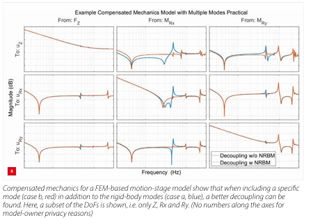
Figure 5 shows thatg when including the non-rigid-body mode, the decoupling ensures that the rigid-body input is not actuating the non-rigid-body mode. In other words, applying this method takes into account that the system is not actually a rigid body and that the actuators are in fact not on the same body. Based on that, a distribution of forces is made that results in a similar movement for all bodies. Additionally, in the off-diagonals we see a better decoupling (lower magnitude) when including the non-rigid-body mode.

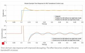
When a step response is obtained with and without decoupling from the non-rigid-body mode, an increase in the achievable bandwidth is shown that also results in better time-domain behaviour performance, as shown in Figure 6.

In summary, when a theoretical model is present, it is possible to obtain the exact eigenmodes of the actuators and the input distribution matrix. A selection can be made from all available modes that should be controlled or decoupled from ^V_I^T ∙ H. The actuator matrix can be calculated as AM = (^V_I^T ∙ H)^–1.

Practical approach

In practice, a measured transfer function is given and the individual masses and internal stiffnesses are often not known. Therefore, an approach has to be defined for obtaining the eigenvectors for the non-rigid-body (NRB) mode, along with obtaining the measured mass matrix ^M_inv–meas as described in the introduction. There are various ways to obtain these, but here a singular-value decomposition is applied to the imaginary part of the measured transfer at the resonance frequency of the targeted mode to obtain the eigenvector, resulting in the eigenvector VI-resonant. For the mass matrix, this procedure is equivalent to today’s practice of taking mass-dominated frequency points of measured MIMO transfer functions as estimates for M_inv–meas.

We now need to find a way to extend this measured matrix to make it square and uniquely invertible, i.e. add an extra row. This row should represent the third DoF we want to decouple, i.e. the resonant behaviour. We suggest adding the eigenvector of the system resonance:

$M_{\text{inv-meas-NRB}} = \begin{bmatrix} M_{\text{inv-meas}} \\ V_{l\text{-resonant}} \end{bmatrix}$

Furthermore, the desired mass-matric M_inv has to be extended on the diagonal (with unity). The compensated mechanics as shown in Figure 7 can be found for actuator matrices including and excluding the non-rigid-body mode.

From this bode plot, the same conclusion can be drawn as from the theoretical approach. By including the non-rigid body mode in the decoupling, the diagonal terms are no longer actuating the non-rigid-body mode, and the decoupling to the off-diagonals has significantly increased.

In summary, this method works in largely the same way as the theoretical approach, only now an estimate for the eigen mode ^V_I-resonant has to be obtained from the frequency response function. We suggest simply using the peak values of one of the rows of the measured TF_raw(ω) at ω = ω_resonance for each input column. Alternatively, an eigenmode estimation method such as singular-value decomposition of ^TF_raw(^ω_resonance) can be used to find an expression for ^V_I^T ∙ H. Using this non-rigid-body mode eigenvector, the measured mass matrix (rigid-body eigenmodes) can be extended.

Full example

Having demonstrated the method for a simple example, it can also be applied to a more complex system. For this, use was made of a high-performance motion-stage model for which the measured transfer functions were generated using a FEM (finite-element method) model. The system is 6-DoF controlled and has an over-actuation of 1 (there is one actuator more than there are con trolled DoFs). This means that if the actuators are positioned correctly, it should be possible to decouple and influence one additional mode on top of the rigid-body modes.

The same method as in the practical approach section
above was applied. Including the first non-rigid-body mode in the decoupling (Figure 8) yields a different decoupling compared to the case in which it not included. From this figure, it can be seen that including mode nr. 7 results in it remaining unactuated.

Experimenting with decoupling from other modes did not always yield a better decoupling, as the ‘obsolete’ actuators were not in a position and/or direction that could significantly affect a mode. In-plane actuators therefore cannot be used to decouple from out-of-plane modes. There is thus a physical understanding as to what this extension of the actuator matrix can achieve. Another risk is that some actuators may exert significant more force than others, causing heating or current saturations.

Conclusion

We have shown that using a pseudo-inverse tells the engineer that there is a design space that can be explored to obtain potentially beneficial results for decoupling. The (pseudo-) inverse property of returning perpendicular vectors can be used not only to decouple rigid-body modes from each other, as it often done currently, but also to decouple from non-rigid-body modes. This provides an opportunity for mechanical and mechatronic engineers to work together in finding optimal actuator locations.

Both a theoretical approach and a practical approach have demonstrated a method to do this for a simple example. Including the non-rigid-body mode in the inverse actuator matrix resulted in a mode disappearing from the measured response without actively controlling it or observing it. Distributing forces such that the mode is not actuated means that there is no energy in that mode, and this no response from the mode is visible. The benefit of this is:

fewer dynamics visible on the diagonals of the system, which potentially allows for higher controller bandwidths;
better decoupling between the logical axes, which
indicates less cross-talk.

From a more advanced model, we could also see that using the design space given by the over-dimensioned system could yield beneficial results. However, we could also conclude that the design space does not always yield beneficial results. The mode to be decoupled (to remain unactuated) has to be within the null-space of the rigid-body modes to be actuated. If this is not the case, undesirable coupling may be the result. Taking this into consideration in the design phase, mechanical design changes and/or changes of actuator locations may improve the situation.

Authors' Note

Mathijs Schouten (mechatronics engineer) and Frank
Sperling (director Technology) work at Nobleo Technology in Eindhoven (NL), an engineering firm specialising in autonomous intelligent systems. Georgo Angelis is a dynamics expert for Nobleo Technology and CEO of Sensing360 in Utrecht (NL).

Frank.sperling@nobleo.nl
www.nobleo-technology.nl
www.sensing360.com

Authors: Mathijs Schouten, Georgo Angelis and Frank Sperling

Reference:

[1] C. Hao et al., “Analysis and Veri cation of Position Error of Reticle Stage Based on Planar Grating”, Laser & Optoelectronics Progress, vol. 56 (23), 231202, 2019.

Dive into the full article Mikroniek 2024-2 – Actuator matrix design

Table of Contents