Validating NN-MPC on a mechatronic system
Model predictive control (MPC) is a well-known technique to tackle challenging control problems. It is based on solving a numerical optimisation problem at every time step to find the best control action. A key drawback of MPC is its computational burden, which hinders industrial application. In this article, we present our approach to approximate MPC solutions using neural networks (NN-MPC), which yields high performance, yet at a strongly reduced computational load and simplified deployment, thereby enabling broader usage in industry.
Introduction
In industry, requirements on accuracy, productivity and/or energy efficiency are continuously increasing. Furthermore, systems are becoming more complex and are being used in more variable conditions. All of these lead to a need for more advanced control. A key method that can tackle these challenging control problems is called Model-Predictive Control (MPC).
MPC is an advanced control technique that, during operation, at every time step, chooses the best control action by solving a numerical optimisation problem [1]. It does so by looking ahead over a given future horizon, while employing predictions of upcoming events and accounting for constraints. This enables the MPC to yield superior performance compared to controllers widely-used in industry, such as PID and LQR controllers.
Typical application areas of MPC are the process industry, building energy systems (HVAC) and energy management [2]. The industrial application of MPC to fast mechatronic systems remains limited however. This is due to one of the key drawbacks of MPC: the computational burden associated with its optimisation. As a result, MPC update rates are limited and/or suffer from deployment challenges on industrial controllers, especially for (i) systems with small time constants, (ii) systems with many states, and/or (iii) systems with highly nonlinear dynamics.
In this work, we present our approach to approximate MPC solutions using neural networks (NN-MPC [3]). We show that the NN-MPC approach yields a high level of performance, reaching nearly the level of the original MPC, yet at a strongly reduced computational load and simplified deployment, thereby enabling broader usage in industry.
Model-predictive control
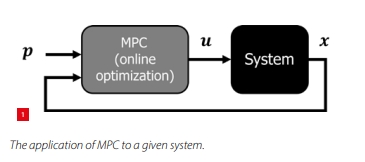
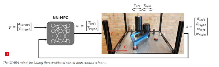
A model-predictive controller employs a model of the system dynamics (which maps the inputs u to states x), allowing to predict the future response of the system. Figure 1 illustrates the application of MPC to a given system. The MPC is a function of the current state x, as well as of certain task-specific parameters p, such as desired initial/final conditions, constraints, predicted variables, etc.
The model-predictive controller has a feedback-like structure. At every time sample, an optimisation problem is solved that calculates the (predicted) optimal input over a given future horizon, according to a model, cost function and constraints. Once the optimal control inputs are computed, only the inputs corresponding to the first sample are applied to the system. After doing so, the new system’s state x is observed, and the MPC is solved for the next time step (starting from the new state). This enables the controller to be robust against model-plant mismatches and disturbances. Furthermore, through employing predictions, MPC can anticipate to upcoming events like disturbances or varying loads.
Approach: NN-MPC
Our proposed approach to approximate MPC solutions using neural networks consists of three steps. The first two steps (dataset generation and training of the network) are computationally demanding, but can be performed before deployment. During deployment (the third and final step), only inference of the neural network is performed, which has limited computational demands and can therefore be executed in real-time
1. Dataset generation
Offline, we solve a large set of MPC problems. The goal is to capture the desired operating region of the system, in terms of the states x, and the subset of task-specific parameters/conditions/predictions p that are expected to vary during operation.
For each of the MPC solutions, all MPC inputs (states x and conditions p) are stored in dataset X. The corresponding optimal control actions (corresponding to the first sample) computed by the MPC are stored in dataset U. The richer the datasets, the better the approximate controller will perform in a variety of (un)seen conditions, but the higher the computational effort required to build the dataset and to train the neural network.
2.Training neural network
Still offline, we train a neural network that aims to approximate the mapping from the input features (dataset X) to the output features (dataset U), as depicted in Figure 2.
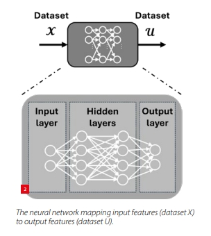
Typically, we consider a feedforward neural network, due to its general-purpose nature. An example of such a network is shown on the right in Figure 2. The network consists of multiple layers. The first part of the network is the input layer, which contains the input features. The second part of the network contains the hidden layers. The complexity of this part of the network can be modified according to the considered use case, by adapting the number of hidden layers as well as the number of neurons per layer. The final layer is the output layer, which converts the information from the hidden layers to the output features (i.e., the control actions).
In the figure, each circle represents a neuron: it receives information from the previous layer and passes it to the next. Within each neuron, the incoming signals are combined after being weighted, and a bias term is added. The result of this calculation is then fed through an activation function (e.g., ReLU or Tanh), which enables the network to decide which neurons become active, and which do not, enabling complex patterns to be captured.
After the architecture of the network is defined, it can be trained by optimising these weights and biases. In this case, we construct the networks using PyTorch and use an Adam optimiser to optimise the weights and biases [4]. The cost function used to train the black-box model is the mean squared error between the output features in U and the predictions of the network. After scaling the input and output datasets, the training is run for a number of epochs until the fitting error is sufficiently low.
3. Deployment
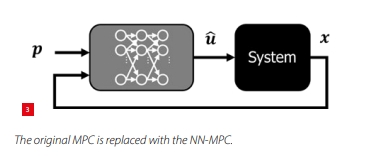
At run-time, the neural network is used to calculate the NN-MPC control input û based on the current inputfeatures (x and p), and is deployed as a direct replacement to the original MPC controller, as shown in Figure 3.
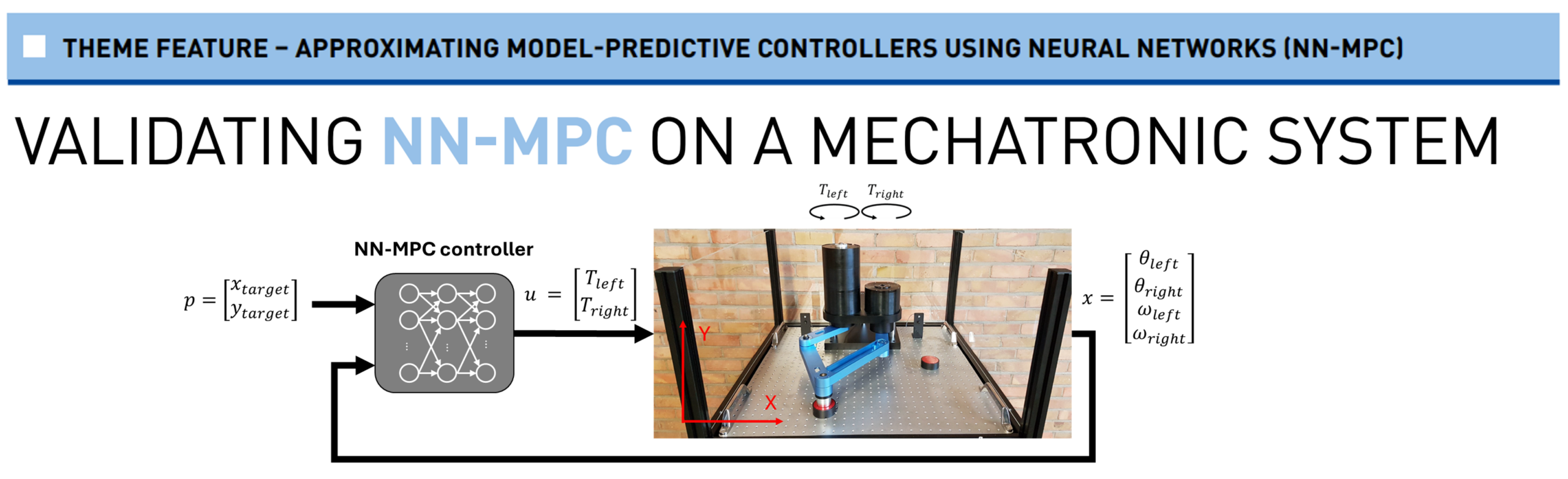
Application to SCARA robot
The approach is applied to a high-speed parallel SCARA robot (see Figure 4). Such a SCARA robot is often used for pick & place or assembly operations, where high velocities and high accuracy are required.
The system is driven by two torque-controlled motors (two inputs u = [Tleft, Tright ]), which control the location and speed of the end-effector in the X-Y plane (four states x = [θleft, θright, ωleft, ωright], where θ denotes the angle and ω the angular velocity). The system has a low time constant, pronounced nonlinear dynamics, various constraints, and has multiple inputs and multiple outputs (MIMO), making it challenging to control. A (multi-body) model of the system is created using Robotran [5], which can be used to generate the MPC solutions.
In the next sections, first a simulation study is conducted and second, the results are validated experimentally.
Simulation study
In this section, the proposed approach is validated in simulation. The control goal of the MPC is to perform a point-to-point motion, from a varying initial end-effector state to a varying final end-effector state, while minimising the required input torque. Furthermore, the end-effector has to avoid a fixed circular obstacle. For this simulation study, we consider a sampling time of 2.5 ms and a total task length of 0.25 seconds (100 samples). However, as the task is executed, each time, the length of the remaining MPC horizon is decreased by 1, going from 100 initially down to 1 as the task is completed.
First, we construct the input and output dataset, by varying the initial and final end-effector positions. In total, we have generated a dataset of 4,096 configurations. For this study, the considered initial and final positions are equidistantly sampled in the considered operating region. For MPC control actions that are varying relatively smoothly over the operating range, such a simple sampling approach suffices. However, when more discrete changes in control actions occur, more intelligent sampling is required. Future work will investigate methods that aim to sample the operating region more efficiently, thereby reducing the training data requirements, while maintaining performance.
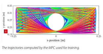
All trajectories, including the obstacle, are visualised in Figure 5, where it can be seen that the training data covers the region of interest densely. Neural networks are known to interpolate correctly in their training domain, but extrapolation on samples that stand farther away from this domain is not guaranteed to perform well [6]. By sampling the operating region densely for the training dataset and by executing tasks within this operating region during deployment (i.e., interpolation), we can expect the neural network to approximate the MPC control actions well.
Second, we construct a neural network consisting of two fully connected hidden layers with 150 neurons, and ReLU activation functions. The inputs to the neural network are the current state (x) and conditions (p), which consist of the desired final positions of the end-effector, as well as the (integer) number of samples remaining until the end of the
total task horizon. This last feature provides a notion of how much time the (NN-)MPC has left to finish the task. The outputs are the two predicted motor torques (û). The neural network is trained until the fitting error on the training dataset is sufficiently low.
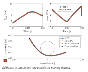
Third, the trained neural network is deployed as a replacement of the original MPC. For validation, we consider a case where the initial and final conditions are placed relatively far away from the initial and final conditions seen in the training dataset (but within the region of interest, i.e., interpolation), aiming to investigate how well the proposed algorithm generalises to unseen data. The result is shown in Figure 6; the solutions are still very similar. With respect to the cost function, the original MPC has an RMS torque of 0.660 Nm, while the NN-MPC has an RMS torque of 0.662 Nm.
Regarding evaluation time: evaluating the original MPC takes 40 ms per iteration (on average), while the MPC approximation only requires 0.5 ms per iteration (in this case, limited by the non-real-time PC operating system used). Hence, the proposed approach speeds up the calculation time in simulation by almost a factor 100 (and allows the controller to be implemented well within the considered sampling time of 2.5 ms).
Experimental validation
In this section, the proposed approach is validated experimentally. A similar workflow is followed as for the simulation study: we consider again a point-to-point task, in this case with a time horizon of 0.3 s, and a sampling frequency of 1 kHz.
However, in contrast to the simulation study, it is expected that the dynamics of the model used to generate the MPC solutions are no longer perfectly equal to the dynamics of the system to which the (NN-)MPC is deployed. The higher this model-plant mismatch, the more the solutions in the training dataset will deviate from the true optimal behaviour, and the more the (NN-)MPC has to correct for the effects of this mismatch during deployment.
The training dataset consists of 625 trajectories from one state to the next (187.5K samples in total). This training data is generated using a (single) nominal model which is fitted (a priori) to measurements of the true system, aiming to reduce the initial model mismatch. In order to deal with the effects of the remaining mismatch, the original dataset is augmented with another dataset of 500 trajectories with 30 samples each (15K in total). This latter dataset consists of several trajectories with a small displacement around the final positions, ‘teaching’ the NN-MPC to correct for the effects of remaining mismatch (similar to a feedback controller).
As an alternative approach, we could have augmented the training dataset with data generated using various (perturbed) versions of the model and let the network find the best match during operation, which will be studied in future work.
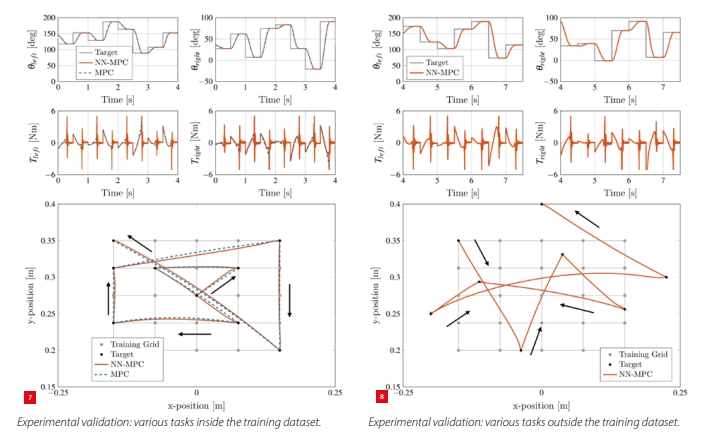
Employing the above dataset, the neural network, as described in the previous section, is trained. After training the NN-MPC, it is applied to the experimental set-up as a direct replacement of the original MPC. In Figure 7, the results are shown for eight point-to-point tasks that are direct members of the training dataset. On the left, the joint angles θleft and θright are shown, as well as the resulting torques T left and T right. On the right, the resulting displacements in Cartesian space are shown, as well as the grid on which the training data is sampled.
The following observations are made:
- For each of the considered tasks, the NN-MPC successfully moves from the initial grid point to the target grid point. At the designated final time of each task (i.e., after 0.3 s), the mean absolute error in Cartesian space is 0.43 mm (approximately 0.4% of the total Cartesian displacement).
- The joint angles and Cartesian displacements computed by the NN-MPC match the original MPC results well. Note however: the results shown for the original MPC are those corresponding to the training dataset (i.e., simulation) only, since the original MPC cannot be deployed directly on the experimental set-up due to its high calculation time, preventing direct comparison.
- The motor torques of the NN-MPC match quite well with those in the training data (MPC). However, towards the end of the motion, the NN-MPC makes more aggressive corrections to ensure the final point is reached and the end-effector comes to standstill. This behaviour is also expected to occur for the MPC performing such a motion under the same model-plant mismatch: it is an effect of the hard constraint on the MPC target position. Improvements can be made by reducing the model-plant mismatch and/or by adapting the original MPC: by re-tuning the cost function, or by adding some slack to the final constraint of the MPC to yield trajectories with smoother torque profiles near the target.
Figure 8 shows the results for seven point-to-point tasks outside the training dataset. The first few tasks ‘interpolate’ within the training grid, and the latter three tasks even go outside the training grid. Again, the NN-MPC successfully performs the motion from each grid point to the next, even when ‘extrapolating’ beyond the seen grid points. At the designated final time of each task (i.e., after 0.3 s), the mean absolute error in Cartesian space is 0.40 mm (approximately 0.3% of the total Cartesian displacement), confirming the NN-MPC generalises well to unseen conditions (for this use case and application).
Regarding evaluation time: recall that evaluating the original MPC takes 40 ms per iteration (on average). For the NN-MPC (in this case deployed on a Beckhoff real-time target), the full loop time (reading encoders, inference of neural-network, sending new torques, …) is reduced to ~8 μs, which is a speed up of a factor 5,000!
Conclusion and ongoing work
The proposed approach enables advanced controllers (MPC) to be implemented on highly dynamic applications, through approximation using neural networks. The approach is applicable to various tasks and systems, for which the operating region and conditions are defined/can be captured within a training dataset. Experimental validation has shown that improvements in calculation speed of up to a factor of 5,000 are achievable, and that the performance of the original MPC is approached.
Ongoing work focuses on a range of topics:
- Efficient generation of the datasets.
- Dealing with varying system dynamics and/or model-plant mismatch through implicit system identification.
- Enhancing extrapolatability to unseen conditions.
- Further experimental validation.
Authors' Note
The authors are associated with Flanders Make in Leuven (BE), the Flemish strategic research centre for the manufacturing industry. Jeroen Willems is also working at Nobleo Technology in Eindhoven (NL) as a control engineer/mechatronics designer.
This work was carried out in the framework of Flanders Make’s SBO projects DIRAC_SBO and LearnOpTra_SBO, funded by Flanders Make, and the AI Research Program, funded by the Flemish Government.
edward.kikken@flandersmake.be
jeroen.willems@nobleo.nl
www.flandersmake.be
www.nobleo-technology.nl
Authors: Jeroen Willems, Edward Kikken, Maxime Monsieur, Andrea Giusti, Branimir Mrak and Bruno Depraetere
References
[1] J.A.E. Andersson, et al., “CasADi – A software framework for nonlinear optimization and optimal control”, Mathematical Programming Computation, 2019.
[2] M. Schwenzer, et al., “Review on model predictive control: An engineering perspective”, The International Journal of Advanced Manufacturing Technology, vol. 117 (5), pp. 1327-1349, 2021.
[3] E. Kikken, et al., “Approximating MPC solutions using Neural Networks; Towards Application in Mechatronic Systems”, Benelux Meeting on Systems and Control, 2024.
[4] A. Paszke, “PyTorch: An imperative style, high-performance deep learning library”, arXiv preprint, arXiv:1912.01703, 2019.
[5] N. Docquier, et al., “Robotran: a powerful symbolic generator of multibody models”, Mechanical Sciences, vol. 4 (1), pp. 199-219, 2013.
[6] A. Courtois, et al., “Can neural networks extrapolate? Discussion of a theorem by Pedro Domingos”, Revista de la Real Academia de Ciencias Exactas, Físicas y Naturales. Serie A. Matemáticas, vol. 117 (2): 79, 2023.
Read the full article here: Mikroniek 2025-6 – NN-MPC (1)
Interested in learning more about how we can collaborate? Visit one of our mechatronics expertise pages for more information: Advanced mechatronic development, system dynamics & control, precision engineering, or systems engineering. Or contact us directly by filling out the contact form below.